深度学习系列(六):YOLOv3算法理论

YOLO v1 至 v2 简介

YOLO v1

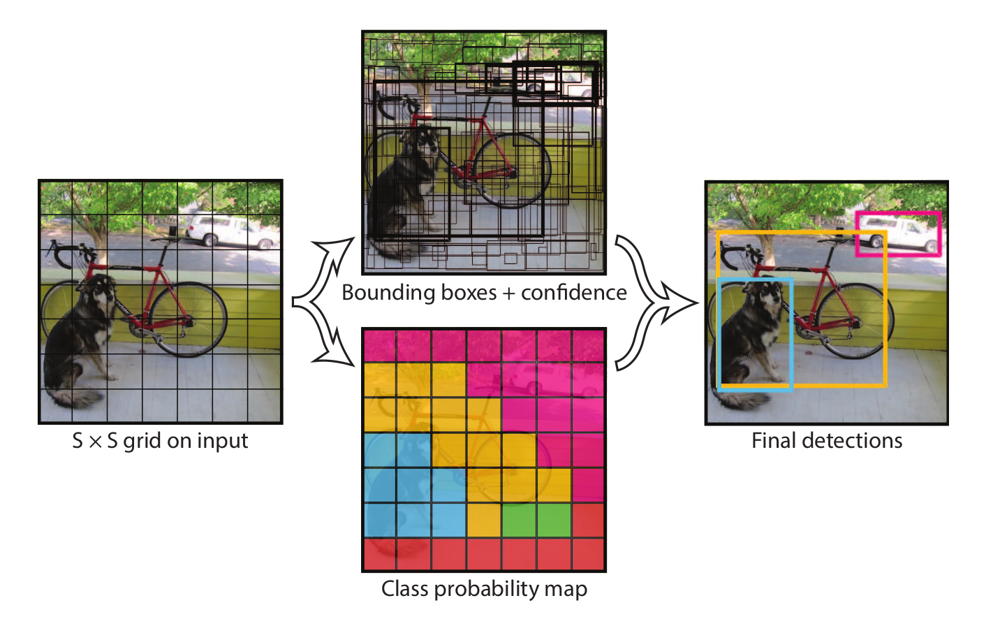
You Only Look Once: Unified, Real-Time Object Detection 在 2016 年被提出，相比于 Faster RCNN 算法，其思路和结构更加简单，能够以实时的推理速度对图片进行目标检测，且能够在标准数据集上达到较好的检测效果。该算法被提出后，受到目标检测领域的广泛关注。

YOLO v1 将目标检测问题视为一个简单的回归问题，其将输入图片均匀地切成 $S \times S$ 的网格，当真实目标的中心点落在某个网格中时，这个网格就负责预测这个目标。每个网格负责预测 $B$ 个 Bounding Box 的参数，包括其中心点坐标和宽高： $x, y, w, h$ ，以及目标置信度 $conf$ ，其中置信度代表目标框和真实框之间的 IOU。除此之外，每个网格还负责预测 $C$ 个数值，用于表示当前目标所属的类别， $C$ 为目标类别数。网络最终预测的张量形状为 $S \times S \times (B * 5 + C)$ 。

对于原论文来说，其将图片分为 $7 \times 7$ 大小的网格，每个网格预测 $2$ 个目标框，PASCAL VOC 数据集共有 $20$ 个目标类型。因此网络最终的预测为一个 $7 \times 7 \times 30$ 的张量。

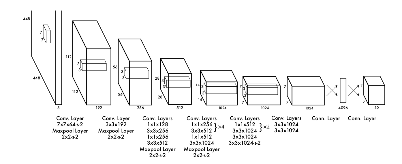
YOLO v1 使用的网络是受 GoogLeNet 启发而设计的一个卷积神经网络。其结构如下：

YOLO v1 的损失函数设计也十分巧妙，这里就不详细说明了，只是基本介绍 YOLO v1 算法的基本思想，在本节开头给出的原论文中有详细的介绍。

YOLO v2

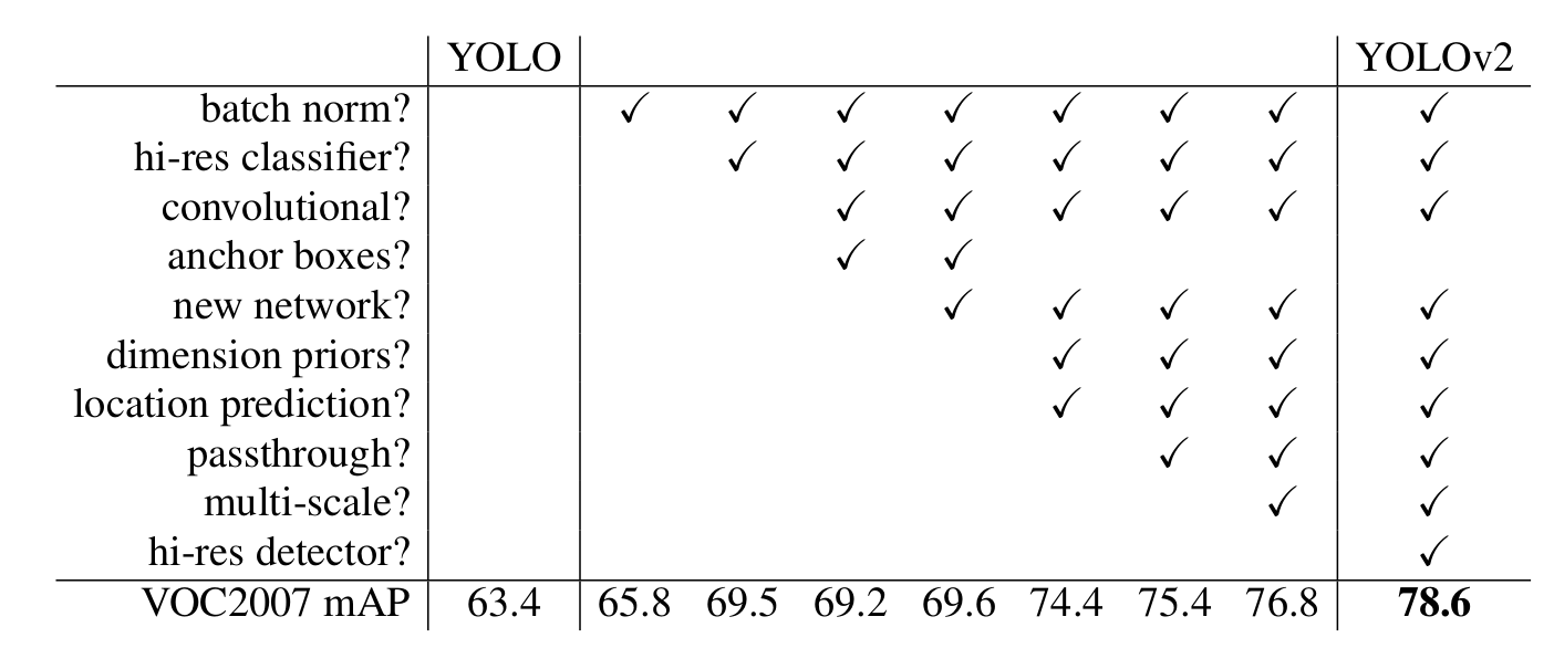
YOLO9000: Better, Faster, Stronger是 YOLO v1 原作者对其算法的改进，一般也被称为 YOLO v2，从论文标题也能看出，改进后的算法更加的快、更加的好、识别的对象也更多。

总结来说，YOLO v2 做出了以下几点改进：

下面分别简单介绍：

Batch Normalization

也叫批量归一化，这已经是当前卷积神经网络中普遍运用的一个手段了，可以对网络起到一定的正则化效果，通常在卷积层操作之后对下一层的输入作批量归一化操作，从而能够得到更好的收敛速度和效果。

High Resolution Classifier

YOLO v1 中使用的网络是在 ImageNet 上预训练得到的，网络的输入分辨率为 224*224，而最终目标检测网络的输入图片分辨率为 448 * 448，这样分辨率切换并不是很友好，YOLO v2 对 YOLO v1得到的网络再使用 448 * 448 的高分辨率图片进行了微调，这样得到了更好的准确率。

Convolutional With Anchor Boxes

YOLO v1 是无锚框的目标检测算法，每个网格直接预测目标的中心点坐标和宽高。YOLO v2 借鉴 Faster RCNN 算法的思想，在每个网格设定一系列不同大小和宽高的锚框，网络负责预测锚框调整参数，采用锚框之后，算法的精度为稍微下降，但是召回率有很大的提高。

Dimension clusters

上面设定的锚框尺寸是手动选择的（就像Faster RCNN算法一样），YOLO v2尝试找到更加科学的锚框尺寸，减少调整参数预测难度。其先对数据集中真实目标框进行聚类，得到最终更好的预设定锚框尺寸。

Direct location prediction

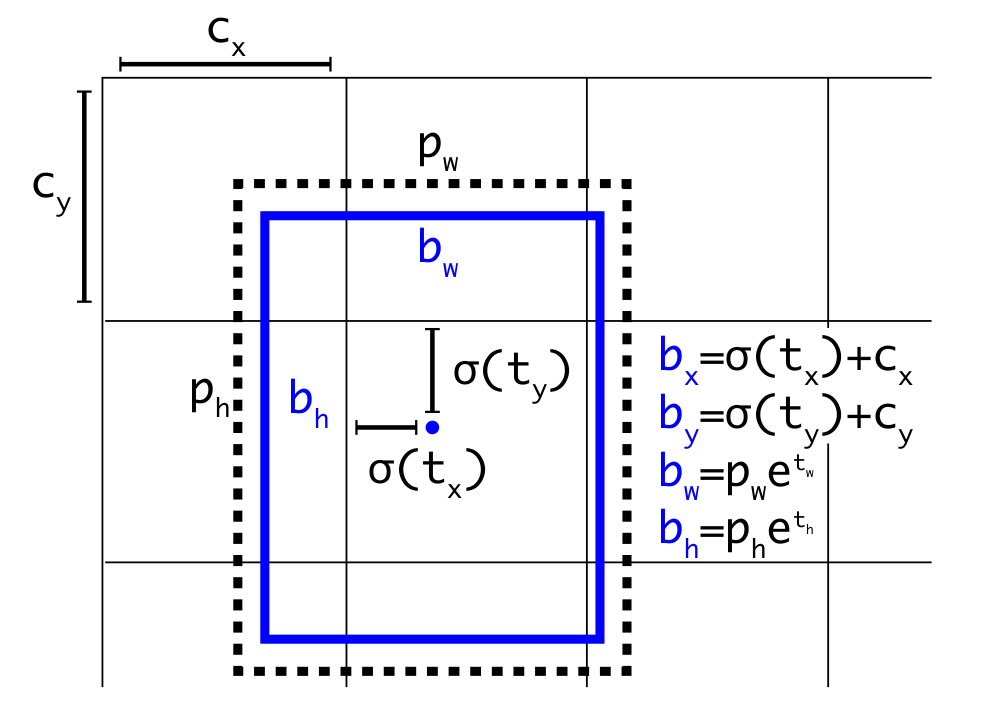
使用预设定锚框会使网络变得不稳定，因为网络预测参数不会预测调整量。因此 YOLO v2 让网络预测锚框的调整参数 $t_x, t_y, t_w, t_h$ ，最终的预测结果计算如下：

Fine-Grained Features

网络对输入图像进行了较大倍率的下采样，这样小目标的特征可能被忽略了，YOLO v2 采用一些 passthrough 层对特征图细节信息进行保留。

Multi-Scale Training

作者在网络训练的时候，每一定的 epoch 之后采用不同尺寸的图像进行输入，从而让网络适应不同大小的图片。

此外，神经网络的结构也不同，YOLO v2采用一个新的卷积神经网络：Darknet19，在ImageNet分类任务中，该网络能够取得非常好的表现，且网络的计算量相较于同准确度的 ResNet 更低。

YOLO v3 原理

实际上，我认为 YOLO v2 和 Faster RCNN 中的 RPN 网络十分相似，就像是 RPN 网络的多分类版本，但是在网络 Backbone 的设计上有所不同。下面详细介绍一下算法原理，并附上部分代码。而 YOLO v3 进一步修改了主干网络，且针对不同尺度目标检测设计了FPN结构。

YOLO v3 论文写得十分随意，但也不影响其获得巨大的引用量。

网络结构

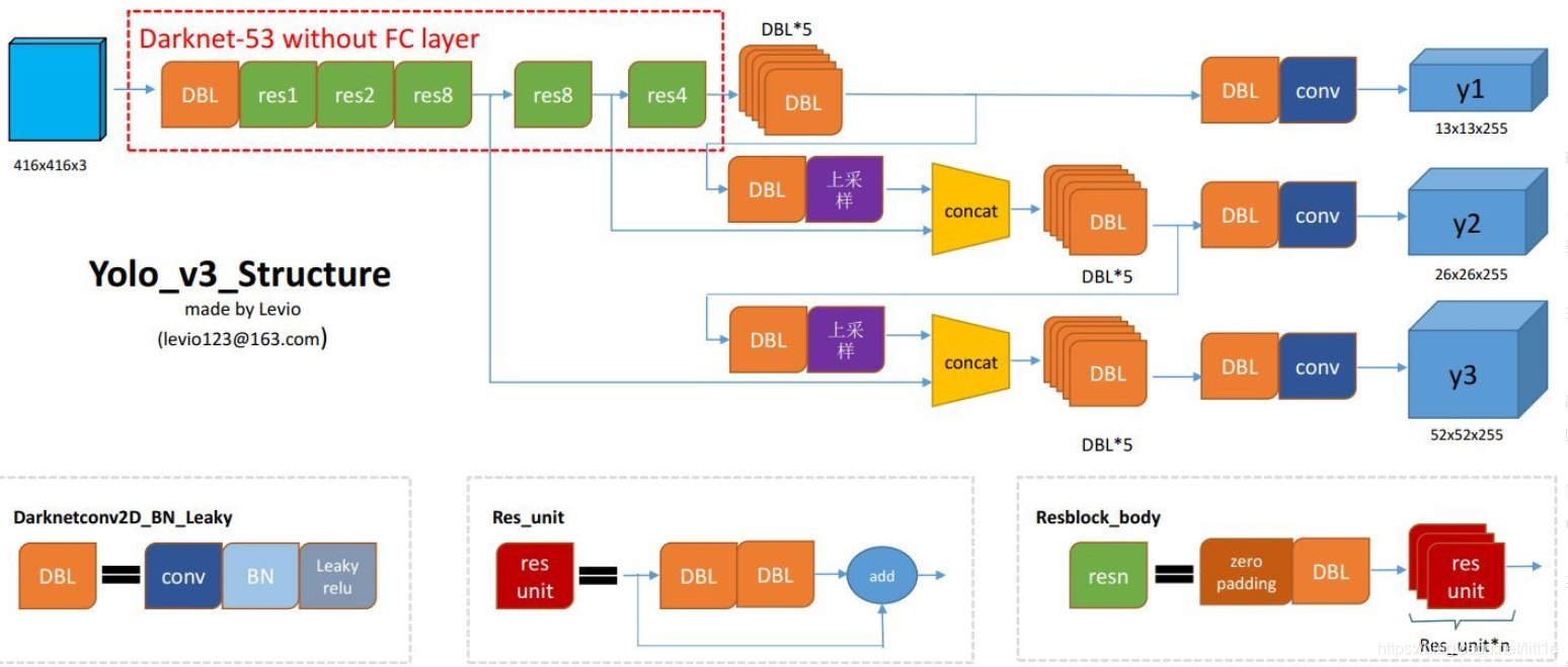
关于网络结构，较难从原论文中得出，这里找到一张十分清楚的网络结构图，出处如下：https://blog.csdn.net/leviopku/article/details/82660381

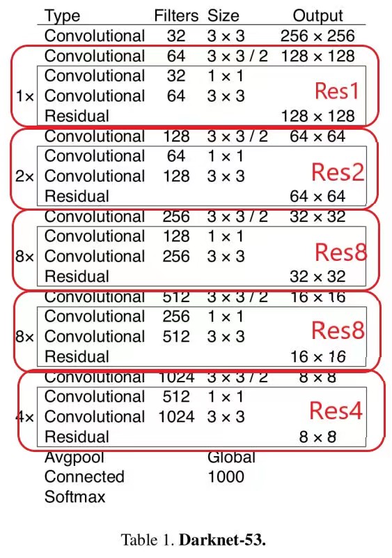
网络的主干为 Darknet53，是 YOLO v2 中Darknet19的进阶版本，性能更加优秀。Darknet53 的具体结构如下：

图中的Res1, Res2等分别对应上面结构图中的。可以看出 YOLO v3 在 Darknet53 取了三个不同深度处的输出，分别是原图 8 倍下采样、16 倍下采样和 32 倍下采样的特征图。

Darknet53的pytorch实现如下：

import math
from torch import nn
from collections import OrderedDict


class ResidualBlock(nn.Module):
    """
    in_channel(int):
    out_channels(List[int]):
    """
    def __init__(self, in_channel, out_channels):
        super().__init__()
        self.conv1 = nn.Conv2d(in_channel, out_channels[0], kernel_size=1, stride=1, padding=0, bias=False)
        self.bn1 = nn.BatchNorm2d(out_channels[0])

        self.conv2 = nn.Conv2d(out_channels[0], out_channels[1], kernel_size=3, stride=1, padding=1, bias=False)
        self.bn2 = nn.BatchNorm2d(out_channels[1])

        self.relu = nn.LeakyReLU(0.1)

    def forward(self, x):
        identity = x
        out = self.conv1(x)
        out = self.bn1(out)
        out = self.relu(out)

        out = self.conv2(out)
        out = self.bn2(out)
        out = self.relu(out)

        out += identity

        return out

    
class Darknet(nn.Module):
    def __init__(self, layers):
        super().__init__()
        self.inplanes = 32
        self.conv1 = nn.Conv2d(3, self.inplanes, kernel_size=3, stride=1, padding=1, bias=False)
        self.bn1 = nn.BatchNorm2d(self.inplanes)
        self.relu1 = nn.LeakyReLU(0.1)

        self.layer1 = self._make_layer([32, 64], layers[0])
        self.layer2 = self._make_layer([64, 128], layers[1])
        self.layer3 = self._make_layer([128, 256], layers[2])
        self.layer4 = self._make_layer([256, 512], layers[3])
        self.layer5 = self._make_layer([512, 1024], layers[4])

        self.layers_out_filters = [64, 128, 256, 512, 1024]

        # weight init
        for m in self.modules():
            if isinstance(m, nn.Conv2d):
                n = m.kernel_size[0] * m.kernel_size[1] * m.out_channels
                m.weight.data.normal_(0, math.sqrt(2. / n))
            elif isinstance(m, nn.BatchNorm2d):
                m.weight.data.fill_(1)
                m.bias.data.zero_()

    def forward(self, x):
        x = self.conv1(x)
        x = self.bn1(x)
        x = self.relu1(x)

        x = self.layer1(x)
        x = self.layer2(x)
        out3 = self.layer3(x)
        out4 = self.layer4(out3)
        out5 = self.layer5(out4)

        return out3, out4, out5
        

    def _make_layer(self, planes, blocks):
        layers = []
        layers.append(("ds_conv", nn.Conv2d(self.inplanes, planes[1], kernel_size=3, stride=2, padding=1, bias=False)))
        layers.append(("ds_bn", nn.BatchNorm2d(planes[1])))
        layers.append(("ds_relu", nn.LeakyReLU(0.1)))

        self.inplanes = planes[1]
        for i in range(0, blocks):
            layers.append((f"residual_{i}", ResidualBlock(self.inplanes, planes)))
        return nn.Sequential(OrderedDict(layers))

def darknet53():
    model = Darknet([1, 2, 8, 8, 4])
    return model

将深层输出执行若干 DBL 并上采样后和浅层输出进行融合，也就是 concat 起来，这是多尺度预测网络FPN的思路，将浅层特征和深层特征融合起来能够同时处理大尺度目标和小尺度目标。最终网络输出三个预测特征图，也就是三个张量，对于预测分类数为80的COCO数据集而言，其大小分别为： $13 \times 13 \times 255$ 、 $26 \times 26 \times 255$ 和 $52 \times 52 \times 255$ 。其中每个特征图预测 3 个锚框的参数，也就是 $255 = 3\times(5 + 80)$ ，对于只有 20 个类别的PASCAL VOC数据集而言，网络输出最后一维为 25 。

整个 YOLO 网络结构的实现如下：

from .darknet import darknet53

from collections import OrderedDict
import torch
from torch import nn


def conv_bn_relu(in_channels, out_channels, kernel_size):
    pad = (kernel_size - 1) // 2 if kernel_size else 0
    return nn.Sequential(OrderedDict([
        ("conv", nn.Conv2d(in_channels, out_channels, kernel_size=kernel_size, stride=1, padding=pad, bias=False)),
        ("bn", nn.BatchNorm2d(out_channels)),
        ("relu", nn.LeakyReLU(0.1)),
    ]))

def make_last_layers(channels, in_channel, out_channel):
    return nn.Sequential(
        conv_bn_relu(in_channel, channels[0], 1),
        conv_bn_relu(channels[0], channels[1], 3),
        conv_bn_relu(channels[1], channels[0], 1),
        conv_bn_relu(channels[0], channels[1], 3),
        conv_bn_relu(channels[1], channels[0], 1),
        conv_bn_relu(channels[0], channels[1], 3),
        nn.Conv2d(channels[1], out_channel, kernel_size=1, stride=1, padding=0, bias=True)
    )

class YOLOBody(nn.Module):
    def __init__(self, anchors_mask, num_classes, pretrained=False):
        super().__init__()
        
        self.backbone = darknet53()
        if pretrained:
            self.backbone.load_state_dict(torch.load("darknet53.pth"))

        # [64, 128, 256, 512, 1024]
        out_channels = self.backbone.layers_out_filters

        self.last_layer0 = make_last_layers([512, 1024], out_channels[-1], len(anchors_mask[0]) * (num_classes + 5))

        self.last_layer1_conv = conv_bn_relu(512, 256, 1)
        self.last_layer1_upsample = nn.Upsample(scale_factor=2, mode='nearest')
        self.last_layer1 = make_last_layers([256, 512], out_channels[-2] + 256, len(anchors_mask[1]) * (num_classes + 5))

        self.last_layer2_conv = conv_bn_relu(256, 128, 1)
        self.last_layer2_upsample = nn.Upsample(scale_factor=2, mode='nearest')
        self.last_layer2 = make_last_layers([128, 256], out_channels[-3] + 128, len(anchors_mask[2]) * (num_classes + 5))

    def forward(self, x):
        x2, x1, x0 = self.backbone(x)
        out0_conv5l = self.last_layer0[:5](x0)
        out0 = self.last_layer0[5:](out0_conv5l)

        x1_in = self.last_layer1_conv(out0_conv5l)
        x1_in = self.last_layer1_upsample(x1_in)
        x1_in = torch.cat([x1_in, x1], 1)
        out1_conv5l = self.last_layer1[:5](x1_in)
        out1 = self.last_layer1[5:](out1_conv5l)

        
        x2_in = self.last_layer2_conv(out1_conv5l)
        x2_in = self.last_layer2_upsample(x2_in)
        x2_in = torch.cat([x2_in, x2], 1)
        out2 = self.last_layer2(x2_in)

        return out0, out1, out2

对于 YOLO v3，对每张输出特征图生成 3 个锚框，对于尺寸为 $13 \times 13$ 的输出，其检测的目标为大目标，生成的锚框尺寸为： $116 \times 90, 156 \times 198,373 \times 326$ ，对于尺寸为 $26 \times 26$ 的输出，生成的锚框尺寸为： $30 \times 61, 62 \times 45, 59 \times 119$ ，对于尺寸为 $52 \times 52$ 的输出，其检测的目标为小目标，生成的锚框尺寸为 $10 \times 13, 16 \times 30, 33 \times 23$ 。

例如，对于 $13 \times 13$ 大小的输出，其中心点像素生成的锚框如下：

和 YOLO v2 一样，网络预测锚框的调整参数 $t_x, t_y, t_w, t_h$ ，为了得到最终的预测框坐标，需要按照以下公式计算：

b_x = \sigma{(t_x)} + c_x \\ b_y = \sigma{(t_y)} + c_y \\ b_w = p_w * e^{t_w} \\ b_h = p_h * e^{t_h}

其中， $c_x,c_y$ 为当前网格左上角的坐标， $t_w,t_h$ 为生成的锚框的宽和高， $\sigma$ 为sigmoid函数，可以将网络的预测参数映射到 0-1 之间。

得到若干预测框之后，需要进行非极大值抑制操作，这和Faster RCNN网络一样，就不过多介绍了，实际上只要是基于锚框的目标检测算法，都需要进行非极大值抑制操作。

损失函数设计

实际上，网上有很多版本不同的 YOLO v3 实现，且后续版本的 YOLO 算法对损失函数还有改变，这里介绍一下https://github.com/eriklindernoren/PyTorch-YOLOv3的损失函数实现。

def compute_loss(predictions, targets):
    device = targets.device
    lcls, lbox, lobj = torch.zeros(1, device=device), torch.zeros(1, device=device), torch.zeros(1, device=device)
    tcls, tbox, indices, anchors = build_targets(predictions, targets)
    BCEcls = nn.BCEWithLogitsLoss(pos_weight=torch.tensor([1.0], device=device))
    BCEobj = nn.BCEWithLogitsLoss(pos_weight=torch.tensor([1.0], device=device))

    # Calculate losses for each yolo layer
    for layer_index, layer_predictions in enumerate(predictions):
        # Get image ids, anchors, grid index i and j for each target in the current yolo layer
        b, anchor, grid_j, grid_i = indices[layer_index]
        batch_size, _, feat_w, feat_h = layer_predictions.shape
        layer_predictions = layer_predictions.view(batch_size, len(HYP.anchor[layer_index]), -1, feat_w, feat_h)\
            .permute(0,1,3,4,2).contiguous()
        # Build empty object target tensor with the same shape as the object prediction
        tobj = torch.zeros_like(layer_predictions[..., 0], device=device)  # target obj
        # Get the number of targets for this layer.
        # Each target is a label box with some scaling and the association of an anchor box.
        # Label boxes may be associated to 0 or multiple anchors. So they are multiple times or not at all in the targets.
        num_targets = b.shape[0]
        # Check if there are targets for this batch
        if num_targets:
            # Load the corresponding values from the predictions for each of the targets
            ps = layer_predictions[b, anchor, grid_j, grid_i]

            # Regression of the box
            # Apply sigmoid to xy offset predictions in each cell that has a target
            pxy = ps[:, :2].sigmoid()
            # Apply exponent to wh predictions and multiply with the anchor box that matched best with the label for each cell that has a target
            pwh = torch.exp(ps[:, 2:4]) * anchors[layer_index]
            # Build box out of xy and wh
            pbox = torch.cat((pxy, pwh), 1)
            # Calculate CIoU or GIoU for each target with the predicted box for its cell + anchor
            iou = bbox_iou(pbox, tbox[layer_index], x1y1x2y2=False, CIoU=True)
            # We want to minimize our loss so we and the best possible IoU is 1 so we take 1 - IoU and reduce it with a mean
            lbox += (1.0 - iou).mean()  # iou loss

            # Classification of the objectness
            # Fill our empty object target tensor with the IoU we just calculated for each target at the targets position
            # tobj[b, anchor, grid_j, grid_i] = iou.detach().clamp(0).type(tobj.dtype)  # Use cells with iou > 0 as object targets
            tobj[b, anchor, grid_j, grid_i] = 1

            # Classification of the class
            # Check if we need to do a classification (number of classes > 1)
            if ps.size(1) - 5 > 1:
                # Hot one class encoding
                t = torch.zeros_like(ps[:, 5:], device=device)  # targets
                t[range(num_targets), tcls[layer_index]] = 1
                # Use the tensor to calculate the BCE loss
                lcls += BCEcls(ps[:, 5:], t)  # BCE

        # Classification of the objectness the sequel
        # Calculate the BCE loss between the on the fly generated target and the network prediction
        lobj += BCEobj(layer_predictions[..., 4], tobj) # obj loss

    lbox *= 0.1
    lobj *= 1.0
    lcls *= 0.5

    # Merge losses
    loss = lbox + lobj + lcls

    return loss

损失函数分为三部分，第一部分为正样本的边界框回归损失，这里采用的是 CIOU 损失，也就是计算当前正样本网格预测的目标框和真实目标框之间的 CIOU(IOU的一种变体)，并使用 $1 - iou$ 作为损失，这样可以使得预测的目标框和真实框之间的IOU不断减小；第二部分为目标置信度的损失，将正样本处的目标置信度设置为 1，其它位置设置为 0，然后计算 BCE 损失；第三部分为分类损失，将正样本类别对应的位置设置为 1，然后计算预测类别和真实类别向量之间的交叉熵。

总结

本文介绍了 YOLO v1 至 YOLO v3 的计算算法思路和原理，并对 YOLO v3 算法网络结构进行了详细介绍，和 Faster RCNN算法中的RPN网络思想很相似。这里，我参照网上多份YOLO v3的代码，实现了一份 YOLO v3 算法：https://github.com/xiaoqieF/my-yolov3，实现上不是严格按照原论文，但是用于理解算法的细节还是比较有帮助。